
Connection 1 of 5
A noisy frame is a weighted mix
At linear step 100 the frame keeps 0.9471 of the clean picture and mixes in 0.3209 of one noise sample. Every channel value of every pixel uses the same two weights.
The red flesh pixel's red value is 0.8824 on the −1 to 1 scale and its noise value is −0.8699, so the noisy value is 0.9471 × 0.8824 + 0.3209 × (−0.8699) ≈ 0.5565.
xₜ = √ᾱₜ × x₀ + √(1 − ᾱₜ) × εRead it as: √ᾱₜ is the picture weight and √(1 − ᾱₜ) the noise weight at step t.
Connection 2 of 5
The squares add to one, not the weights
At step 100, 0.9471 + 0.3209 ≈ 1.27, more than one. The squares are what add to one: 0.8970 + 0.1030 = 1, because ᾱₜ + (1 − ᾱₜ) = 1.
The weights are amplitudes. Squaring them gives variances, and for a unit-variance noise sample the noise variance is exactly 1 − ᾱₜ.
(√ᾱₜ)² + (√(1 − ᾱₜ))² = 1Read it as: Weights as amplitudes, squares as variances.
Connection 3 of 5
Per-step β, cumulative ᾱ
Each step has its own small noise variance βₜ and keeps αₜ = 1 − βₜ of what was there. ᾱₜ multiplies those keeps over every step so far.
For the linear schedule β₂₅₀ ≈ 0.0051, yet after 250 steps ᾱ₂₅₀ ≈ 0.52. The cosine schedule starts with smaller βs (β₂₅₀ ≈ 0.0013), so ᾱ₂₅₀ ≈ 0.85.
αₜ = 1 − βₜ
ᾱₜ = α₁ × α₂ × … × αₜ,  ᾱ₀ = 1
Read it as: The bar means a running product, not an average.
Connection 4 of 5
Two schedules at the same steps
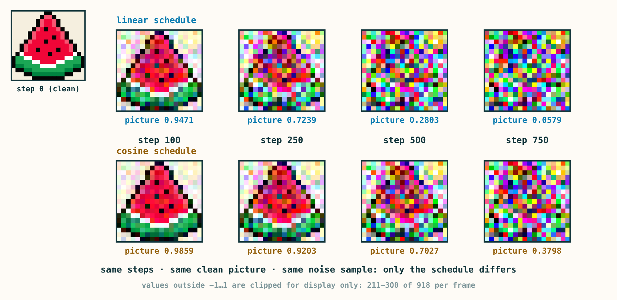
Linear and cosine schedules on the same watermelon and the same noise sample at steps 100, 250, 500 and 750: picture weights 0.9471, 0.7239, 0.2803, 0.0579 against 0.9859, 0.9203, 0.7027, 0.3798.
Linear: βₜ rises in equal steps from 0.0001 to 0.02 over 1000 steps. Cosine: ᾱₜ follows f(t)/f(0) with f(t) = cos²(((t/1000 + 0.008)/1.008) × π/2), so βₜ = 1 − f(t)/f(t − 1), capped at 0.999 at the last step.
With the same noise sample, the picture weights are 0.9471 and 0.9859 at step 100, 0.7239 and 0.9203 at step 250, 0.2803 and 0.7027 at step 500, and 0.0579 and 0.3798 at step 750 (linear, then cosine).
linear: βₜ = 0.0001 + 0.0199 × (t − 1)/999
cosine: βₜ = min(1 − f(t)/f(t − 1), 0.999)
Read it as: Both are fixed rules, chosen before any training; neither is learned.
Connection 5 of 5
Same mix, same look; endpoints are not zero
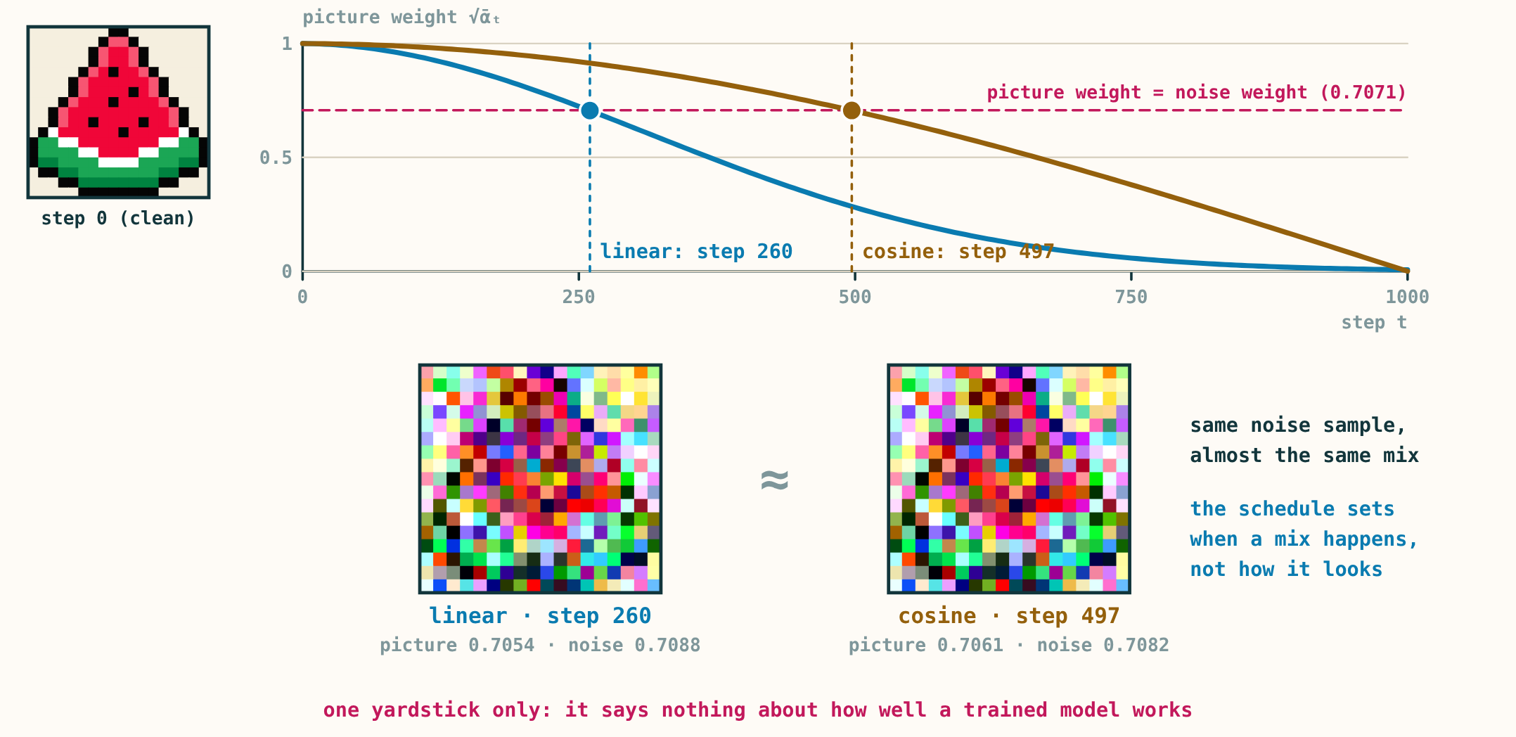
Picture weight across all 1000 steps: the noise weight overtakes at step 260 (linear) and 497 (cosine), and the two crossing frames, built from the same noise sample, look the same.
The noise weight first exceeds the picture weight at step 260 for linear and step 497 for cosine. With the same noise sample, those two frames differ by less than 0.003 in every value: the schedule decides when a mix happens, not how it looks.
At step 1000 the linear schedule still keeps 0.0064 of the picture and the cosine schedule 0.00005. Small, but not zero.
first t with √(1 − ᾱₜ) > √ᾱₜ: 260 (linear), 497 (cosine)Read it as: One yardstick only; it does not say which schedule trains a better model.
Connect it back to the picture
A schedule is a fixed timetable of ᾱₜ. It sets how much picture and how much noise each step holds; it is not a denoiser or a sampler, and which schedule suits a model is found by training, not by looking.
Full notation and technical reference
The expressions below collect the operations discussed above. You can return here when you want the compact notation.
αₜ = 1 − βₜ
ᾱ₀ = 1,  ᾱₜ = α₁ × α₂ × … × αₜ
xₜ = √ᾱₜ x₀ + √(1 − ᾱₜ) ε
linear: βₜ = 0.0001 + 0.0199 (t − 1) / 999
cosine: βₜ = min(1 − f(t) / f(t − 1), 0.999)
f(t) = cos²(((t / 1000 + 0.008) / 1.008) × π/2)- βₜ is the per-step noise variance and ᾱₜ the running product of 1 − βₜ; both schedules use 1000 steps, and step 0 is the clean picture.
- ε is one seeded standard-normal sample (918 values) shared by every compared frame, so differences between frames come only from ᾱₜ. Bytes map to x = byte / 127.5 − 1.
Numerical reference
Linear step 100 keeps √ᾱ = 0.9471 of the picture and mixes in 0.3209 of the noise: the red flesh pixel's red value becomes 0.9471 × 0.8824 + 0.3209 × (−0.8699) ≈ 0.5565. At step 500 the linear schedule keeps 0.2803 and the cosine schedule 0.7027. The noise weight overtakes the picture weight at step 260 (linear) and 497 (cosine).
Where this explanation stops
The compared frames share one ε: a coupled comparison of the distributions at chosen steps, not a step-by-step run of the forward chain. The display clips to −1…1; the model never does. Neither endpoint is exactly zero (picture weight 0.0064 and 0.00005 at step 1000). A schedule is not learned and is neither a denoiser nor a sampler, and looking at frames does not show which schedule trains a better model.